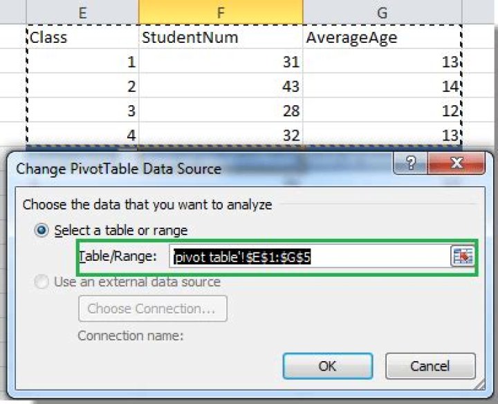
On the Options tab, in the Data group, click Change Data Source, and then click Change Data Source. The Change PivotTable Data source dialog box is displayed. Do one of the following: To use a different Excel table or cell range, click Select a table or range, and then enter the first cell in the Table/Range text box.
How do I edit a calculated field in a pivot table Excel 2007?
Edit a calculated field formula
- Click the PivotTable.
- On the Options tab, in the Tools group, click Formulas, and then click Calculated Field.
- In the Name box, select the calculated field for which you want to change the formula.
- In the Formula box, edit the formula.
- Click Modify.
How do I find the range of a pivot table?
On the Ribbon, under the PivotTable Tools tab, click the Analyze tab (in Excel 2010, click the Options tab). In the Data group, click the top section of the Change Data Source command. The Change PivotTable Data Source dialog box opens, and you can see the the source table or range in the Table/Range box.
How do you create a range in a pivot table?
Group by range in an Excel Pivot Table
- Select the table, and click Insert > PivotTable.
- In the Create PivotTable dialog box, please select a destination range to place the pivot table, and click the OK button.
How do I increase the range of a pivot table in Excel 2007?
Answer:Select the Options tab from the toolbar at the top of the screen. In the Data group, click on Change Data Source button. When the Change PivotTable Data Source window appears, change the Table/Range value to reflect the new data source for your pivot table. Click on the OK button.
How do I filter a calculated field in a pivot table?
1 Answer. You need to select the “Values filter” option from one of the dropdowns you see on the other non-Values PivotField to filter any fields that are in the VALUES area.
Why calculated field is disabled in pivot table?
Drop the data into Excel into a table. If you try to pivot off this data, the calculated field will still be grayed out. BUT, if you make a dynamic range on the table and create a new pivot table that references the dynamic range of the table instead of the table itself, the calculated field will not be grayed out.
How do I see pivot table Field List?
To see the PivotTable Field List:
- Click any cell in the pivot table layout.
- The PivotTable Field List pane should appear at the right of the Excel window, when a pivot cell is selected.
- If the PivotTable Field List pane does not appear click the Analyze tab on the Excel Ribbon, and then click the Field List command.
How do you create a range in Excel?
Another way to make a named range in Excel is this:
- Select the cell(s).
- On the Formulas tab, in the Define Names group, click the Define Name button.
- In the New Name dialog box, specify three things: In the Name box, type the range name.
- Click OK to save the changes and close the dialog box.
How do I change the range of a pivot table?
Excel Pivot Table Update Range 1 After you change the data range, click the relative pivot table, and click Option (in Excel 2013, click ANALYZE ) > Change Data Source . 2 Then in the pop-up dialog, select the new data range you need to update. 3 Click OK . Now the pivot table is refreshed. See More….
How to change data source of relative pivot table in Excel?
1. After you change the data range, click the relative pivot table, and click Option (in Excel 2013, click ANALYZE ) > Change Data Source. See screenshot: 2. Then in the pop-up dialog, select the new data range you need to update.
How to create and edit pivot table in Excel?
Select the table, and click Insert > PivotTable. 2. In the Create PivotTable dialog box, please select a destination range to place the pivot table, and click the OK button. See screenshot: 3. Now go to the PivotTable Fields pane, please drag and drop Score field to the Rows section, and drag and drop Name field to the Values section.
How do you group cells by range in a pivot table?
Group by range in an Excel Pivot Table. With Kutools for Excel’s Advanced Combine Rows feature, you can quick group all cells of one column based on values in another column, or calculate (sum, count, average, max, etc.) these cells by the values in another column at ease!