The IS-LM model has the same horizontal axis as the aggregate demand curve, but a different vertical axis. The LM curve describes equilibrium in the market for money. The LM curve is upward sloping because higher income results in higher demand for money, thus resulting in higher interest rates.
IS-LM and aggregate demand shift in the AD curve?
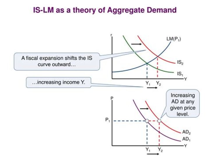
The aggregate demand curve shifts due to any event that shifts the IS curve or the LM curve (when P remains constant). For instance, if M increases Y rises if P remains constant. As a result aggregate demand curve shifts to the right as shown in part (a) of Fig. 11.2.
How do you find the equation of the LM curve?
Algebraically, we have an equation for the LM curve: r = (1/L 2) [L 0 + L 1Y – M/P]. r = (1/L 2) [L 0 + L 1 m(e 0-e 1r) – M/P]. r = A r – B rM/P.
IS-LM model explained?
The IS-LM model appears as a graph that shows the intersection of goods and the money market. The IS stands for Investment and Savings. The LM stands for Liquidity and Money. The IS-LM model attempts to explain a way to keep the economy in balance through an equilibrium of money supply versus interest rates.
Is-LM and AD as model?
The AD-AS and the IS-LM models are equivalent. The IS-LM model relates the real interest rate to output. The AD-AS model relates the price level to output.
Is-LM BP model explained?
In addition to the balance in goods and financial markets, the model incorporates an analysis of the balance of payments. Secondly, the LM curve, which represents the equilibrium in the money market. Thirdly, the BP curve, which represents the equilibrium of the balance of payments.
IS and LM curve equation?
‘ Demand for money is defined by the equation L = kY – hi, where L is the demand for inflation-adjusted money; k is income sensitivity of demand; Y is income; h is interest sensitivity of demand; and i is the interest rate. These factors affect the slope of the LM curve.
Is-LM analysis aggregate demand and supply?
Aggregate demand occurs at the point where the IS and LM curves intersect at a particular price. If some individual considers a higher price level, then the real supply of money will definitely be lower. As a result, the LM curve will shift higher. Furthermore, the aggregate demand will be lower.
How do you calculate aggregate demand?
Aggregate demand equals the sum of consumption (C), investment (I), government spending (G), and net export (X -M). This is often written as an equation, which is given by: AD = C + I + G + (X – M).
Is-LM BP model?
The Mundell–Fleming model, also known as the IS-LM-BoP model (or IS-LM-BP model), is an economic model first set forth (independently) by Robert Mundell and Marcus Fleming. The model is an extension of the IS–LM model.
How is the aggregate demand curve generated from the IS-LM model?
Generating the Aggregate Demand Curve The IS-LM model studies the short run with fixed prices. This model combines to form the aggregate demand curve, which is negatively sloped; hence when prices are high, demand is lower. Therefore, each point on the aggregate demand curve is an outcome of this model.
What is the demand for money in the IS-LM model?
In the IS-LM model we assume that the demand for money is positive function of GDP. As the demand for money depends on Y and R in the IS-LM model, we write MD (Y, R) for the demand for money. Remember that it depends positively on Y and negatively on R.
What is the relationship between aggregate demand and real money supply?
The aggregate demand curve shows the inverse relation between the aggregate price level and the level of national income. Now we may established this relation on the basis of the IS-LM model. Suppose we hold the nominal money supply constant. Now if the price level (P) rises, the supply of real money balances (M/P) falls.
What are the two interpretations of the IS-LM curve?
These curves are used to model the general equilibrium and have been given two equivalent interpretations. First, the IS-LM model explains the changes that occur in national income with a fixed short-run price level. Secondly, the IS-LM curve explains the causes of a shift in the aggregate demand curve.